Getting Started

A walkthrough from pip install to your first plotted spectrum and NIRCam cutout. Running example throughout: RUBIES-EGS-49140 (J141934.14+525238.7) — a Little Red Dot at z=6.69 with public data from RUBIES, CAPERS, EGS-BUBBLES, OCEANS, C3PO, and THRILS.

If you'd rather click "run all" and read the output, the same flow lives in python/examples/quickstart.ipynb.

1. Install#

bash

pip install "git+https://github.com/hollisakins/campfire.git#subdirectory=python/"

For the figures and stacking shown later in this guide, install the optional extras:

bash

pip install "campfire[deploy] @ git+https://github.com/hollisakins/campfire.git#subdirectory=python/"

This pulls in matplotlib, scipy, photutils, reproject, and Pillow — used by NIRCam cutouts, calibration, and stacking. If you only need querying and quick-look plotting, the base install is enough.

2. Authenticate#

bash

campfire login

This opens your browser for OAuth. Approve the device code, and credentials are saved to ~/.campfire/credentials. Tokens auto-refresh; you don't need to log in again unless you campfire logout.

For headless environments (HPC, CI, remote shells without a browser), generate an API key at /profile/api-keys (keys start with sk_) and paste it in:

bash

campfire login --api-key

The same credentials are used by the CLI, the Python client, and any direct REST calls.

3. Sync the catalog#

The catalog lives in a local SQLite database. Sync it once, then query it instantly. Sync is metadata-only — no FITS files yet.

bash

campfire sync

Or, equivalently, from Python:

python

from campfire import Campfire

cf = Campfire()
result = cf.sync()
print(f"Synced {result['observations']} observations, "
      f"{result['objects']} objects, "
      f"{result['spectra']} spectra")

code

Synced 146 observations, 3072 objects, 47340 spectra

Re-running cf.sync() is fast and safe — it updates inspection results, redshifts, tags, and any new spectra. If files have been reprocessed on the server, you'll see a stale-count warning; re-fetch them with cf.download(stale_only=True).

4. The mental model#

Object → SpectrumCollection → Spectrum → SpectrumData. Photometry and tags hang off Object.

Three things to internalise:

query_objects vs query_spectra. An object is one sky position (with inspection state — redshift, redshift_quality, tags). A spectrum is one extraction at that position (with spectrum_id, grating, per-spectrum DQ flags). One object usually has multiple spectra across gratings and programs.
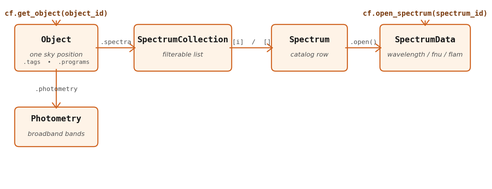
Object is a typed dataclass with everything attached. cf.get_object(object_id) returns an Object whose .spectra is a numpy-style filterable SpectrumCollection, and whose .photometry is a Photometry instance (or None).
SpectrumData is the actual numpy arrays. spec.open() (or cf.open_spectrum(spectrum_id)) reads the FITS file from disk if downloaded, otherwise fetches it from the API and caches it locally.

5. Your first query#

query_objects returns one row per sky position as an astropy.table.Table. Filters can be combined freely.

python

high_z = cf.query_objects(
    redshift_range=(5.0, 12.0),
    redshift_quality=['probable', 'secure'],   # or [3, 4]
    inspected_only=True,
)
print(f"Found {len(high_z)} high-z galaxies")
high_z['object_id', 'field', 'redshift', 'redshift_quality', 'max_snr'][:5]

code

Found 2366 high-z galaxies

     object_id      field  redshift redshift_quality     max_snr
------------------- ----- --------- ---------------- ----------------
J001348.33-301914.6 a2744 10.206251                4  7.7858099937439
J001348.47-301935.7 a2744  7.425598                4 33.1221122741699
J001349.13-301900.8 a2744  9.526492                4 10.6564788818359
J001352.92-301912.4 a2744  7.973281                4 17.3938312530518
J001401.10-301828.5 a2744  7.907672                4 22.6837329864502

The full filter vocabulary (tags, cone search, DQ flags, programs/fields/gratings/observations, photometry status, search) is in the Python Client reference. For a quick taste:

python

# Filter by tag
lrds = cf.query_objects(tags=['lrd'], redshift_quality=['secure'])

# Cone search around a coordinate (RA, Dec, radius_arcsec)
nearby = cf.query_objects(cone_search=(214.892, 52.876, 60.0))

6. Pull a single object together#

python

obj = cf.get_object('J141934.14+525238.7')
print(obj)

code

Object(J141934.14+525238.7, z=6.6900, egs)
  12 spectra (G140H, G140M, G235H, G395H, G395M, PRISM)
  tags: blagn, hae, lrd, o3e
  Photometry(11 bands, UNICORN EGS v0.9)

obj.spectra is a numpy-style filterable container:

python

print(obj.spectra)

code

SpectrumCollection (12 spectra)
spectrum_id                        grating      SNR  exp_time  local
--------------------------------------------------------------------
c3po_p2_g140m_f100lp_46403         G140M       11.3     47268      Y
c3po_p2_g395m_f290lp_46403         G395M      184.6     36764      Y
capers_egs_p3_prism_clear_11585    PRISM      130.0     17069      Y
mason_egs_p3_g140h_f100lp_62859    G140H        4.1     14005      Y
...

python

prism = obj.spectra[obj.spectra.grating == 'PRISM']     # boolean indexing
hi_snr = obj.spectra[obj.spectra.signal_to_noise > 50]  # numeric comparisons

obj.photometry.bands, obj.photometry.flux, etc. give parallel arrays; obj.photometry['f444w'] returns a single band as a (flux, flux_err, wavelength) tuple.

7. Open and plot a spectrum#

SpectrumData.plot() is a one-line quick-look helper. It steps the spectrum and shades a 1-σ error band by default.

python

import matplotlib.pyplot as plt

spec = cf.open_spectrum('capers_egs_p3_prism_clear_11585')
print(spec)
# SpectrumData(capers_egs_p3_prism_clear_11585, PRISM, 419 pixels, 0.55-5.37 μm)

fig, ax = plt.subplots(figsize=(10, 4))
spec.plot(ax=ax)

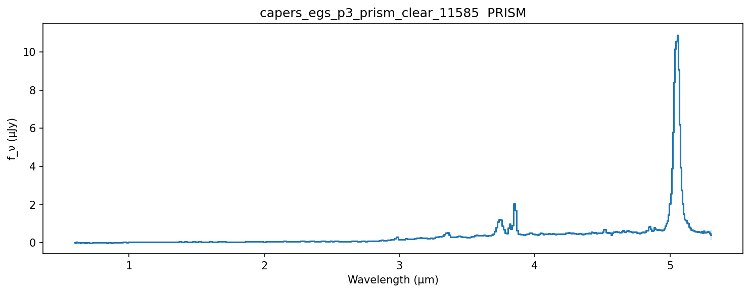
Quick-look PRISM spectrum of RUBIES-EGS-49140 at z=6.69, showing strong emission near 5 μm.

The arrays are also available directly: spec.wavelength (μm), spec.fnu / spec.fnu_err (μJy), spec.flam / spec.flam_err (erg/s/cm²/Å, auto-computed if not in the FITS), spec.header (FITS primary header as a dict).

8. NIRCam cutout#

plot_cutout() produces an RGB image with vector shutter overlays. Both the cutout PNG and shutter geometry are cached locally after the first fetch — subsequent calls are instant.

python

fig, ax = plt.subplots(figsize=(5, 5))
cf.plot_cutout('J141934.14+525238.7', fov=3.2, ax=ax)

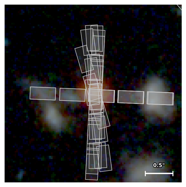
NIRCam RGB cutout of J141934.14+525238.7 with all NIRSpec MOS shutters overlaid.

You can restrict shutters to the target only, or use JADES-style L-shaped corner markers. See the cutout recipe for the full styling vocabulary.

9. Local vs remote#

The client transparently uses local data when available and falls back to the API otherwise:

Operation	If local synced	Otherwise
`cf.query_objects()` / `query_spectra()`	SQLite — unlimited, instant	API — capped at 1000, paginated
`cf.iter_objects()` / `iter_spectra()`	SQLite	API auto-pagination
`cf.get_object(id)` / `cf.get_spectrum(id)`	SQLite	API search fallback
`cf.open_spectrum(id)`	reads local FITS	downloads + caches FITS

cf.is_local tells you which mode you're in; cf.last_synced shows the timestamp. Pass remote=True to any query to force the API path even when synced data is available — useful for verifying that your local copy is current.

Where to go next#

Recipes — six end-to-end task examples: tag-based sample selection, cross-matching, calibration & stacking, large-sample iteration, publication-quality cutouts, SED + spectrum overlay.
Python Client reference — every method and parameter, organised by topic.
CLI Reference — the campfire command-line tool, including bulk download options.