Recipes
Six end-to-end task examples. Each recipe is self-contained and assumes you have already run campfire login + cf.sync() (see Getting Started).
The examples use RUBIES-EGS-49140 (J141934.14+525238.7, public LRD at z=6.69) as a running target where one is needed.
- 1. Build a sample by tag and download its spectra
- 2. Cross-match with an external catalog
- 3. Calibrate and stack a sample
- 4. Iterate over a large sample efficiently
- 5. Publication-quality cutout
- 6. SED + spectrum overlay
1. Build a sample by tag and download its spectra#
Tags are string slugs maintained per-object. Combine them with the standard query filters to define a sample, then call cf.download() to pull the FITS files. Downloads are incremental (SHA-256 checked) and parallel by default.
from campfire import Campfire

cf = Campfire()

# Sample: secure-z Little Red Dots
lrds = cf.query_objects(
    tags=['lrd'],
    redshift_quality=['secure'],
)
print(f"{len(lrds)} secure-z LRDs")

# Pull in only the observations these objects belong to,
# restricted to PRISM gratings
observations = sorted({o for row in lrds for o in row['observations'] if o})
cf.download(observations=observations, gratings=['PRISM'])
Now cf.open_spectrum(spectrum_id) will read from the local FITS for any of these.
To re-fetch reprocessed files after a future cf.sync():
result = cf.sync()
if result['stale_count']:
    cf.download(stale_only=True)
2. Cross-match with an external catalog#
Use astropy's match_to_catalog_sky to attach CAMPFIRE counterparts to your own catalog.
from campfire import Campfire
from astropy.coordinates import SkyCoord
from astropy.table import Table
import astropy.units as u

cf = Campfire()
campfire_egs = cf.query_objects(fields=['egs'])

# Replace with your catalog
external = Table({
    'id':  ['src1', 'src2', 'src3'],
    'ra':  [214.892, 214.880, 214.910],
    'dec': [52.876, 52.880, 52.872],
})

ext_coords = SkyCoord(ra=external['ra'] * u.deg, dec=external['dec'] * u.deg)
cf_coords = SkyCoord(
    ra=campfire_egs['ra'] * u.deg,
    dec=campfire_egs['dec'] * u.deg,
)

idx, sep, _ = ext_coords.match_to_catalog_sky(cf_coords)
matched = sep < 1 * u.arcsec

matches = Table({
    'external_id'      : external['id'][matched],
    'campfire_id'      : campfire_egs['object_id'][idx[matched]],
    'separation_arcsec': sep[matched].to(u.arcsec).value.round(3),
    'redshift'         : campfire_egs['redshift'][idx[matched]],
})
print(matches)
For very small catalogs, cf.query_objects(cone_search=(ra, dec, radius)) per source can be simpler than a full cross-match. For large catalogs, restrict the CAMPFIRE side to the relevant fields first (as above).
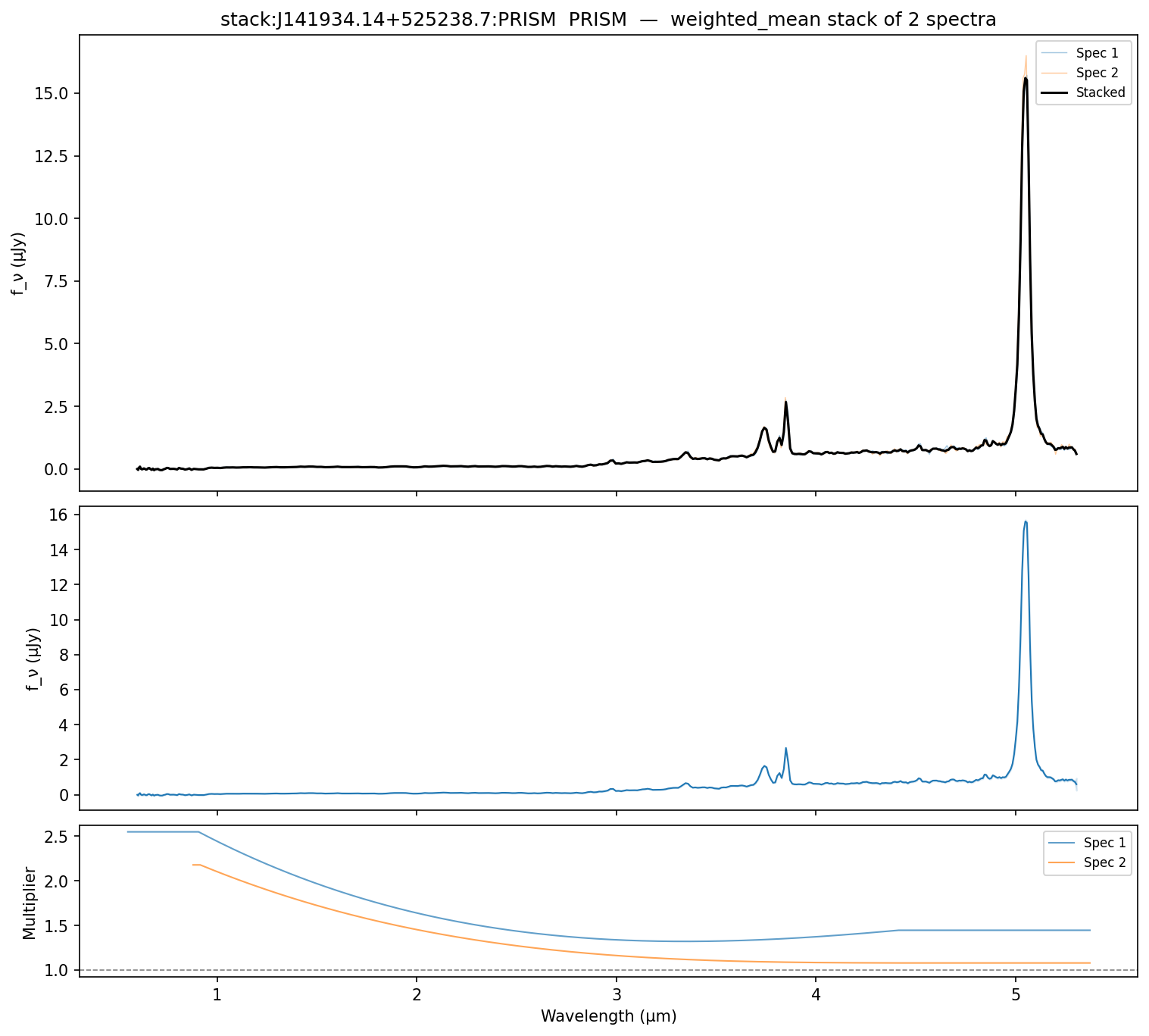
3. Calibrate and stack a sample#
calibrate_and_stack fits a per-spectrum correction (Chebyshev or scalar) so synthetic photometry from each spectrum matches the object's broadband photometry, then resamples and combines them. Useful for combining repeated visits or low-SNR exposures.
Requires the [deploy] extra: pip install -e ".[deploy]".
from campfire import Campfire, calibrate_and_stack

cf = Campfire()
obj = cf.get_object('J141934.14+525238.7')
prism = obj.spectra[obj.spectra.grating == 'PRISM']

result = calibrate_and_stack(
    prism,
    photometry=obj.photometry,
    method='chebyshev',           # 'chebyshev' (default) or 'flat'
    stacking_method='weighted_mean',  # 'weighted_mean' | 'median' | 'mean'
    object_id=obj.object_id,
)

result.spectrum         # SpectrumData — the final stacked spectrum
result.calibrations     # list[CalibrationResult] — per-input fit + diagnostics
result.input_spectra    # list[SpectrumData] — calibrated inputs before stacking
result.plot()           # 3-panel diagnostic
For finer control, the building blocks are also exposed individually: calibrate_to_photometry() calibrates a single spectrum; stack_spectra() combines pre-loaded SpectrumData instances; synthetic_photometry() computes a single AB band flux from a spectrum.
4. Iterate over a large sample efficiently#
iter_objects() / iter_spectra() stream rows one at a time — no full-table materialisation, no pagination bookkeeping. Use them when the result set is large or when you want to short-circuit.
from campfire import Campfire, DQFlags

cf = Campfire()

# Walk every Hα emitter without loading them all into memory
n_inspected = 0
for row in cf.iter_objects(tags=['hae']):
    if row['redshift_quality'] >= 3:
        n_inspected += 1
print(f"{n_inspected} secure/probable Hα emitters")

# Walk clean PRISM spectra, stop after 50 hits
hits = []
for row in cf.iter_spectra(
    gratings=['PRISM'],
    inspected_only=True,
    dq_flags=~DQFlags.CONTAMINATION & ~DQFlags.LOW_SNR,
):
    hits.append(row)
    if len(hits) >= 50:
        break
Combine with cf.open_spectrum(row['spectrum_id']) to pull FITS arrays one at a time. If you find yourself iterating to read many spectra from the API, run cf.download() first so subsequent reads come from local disk.
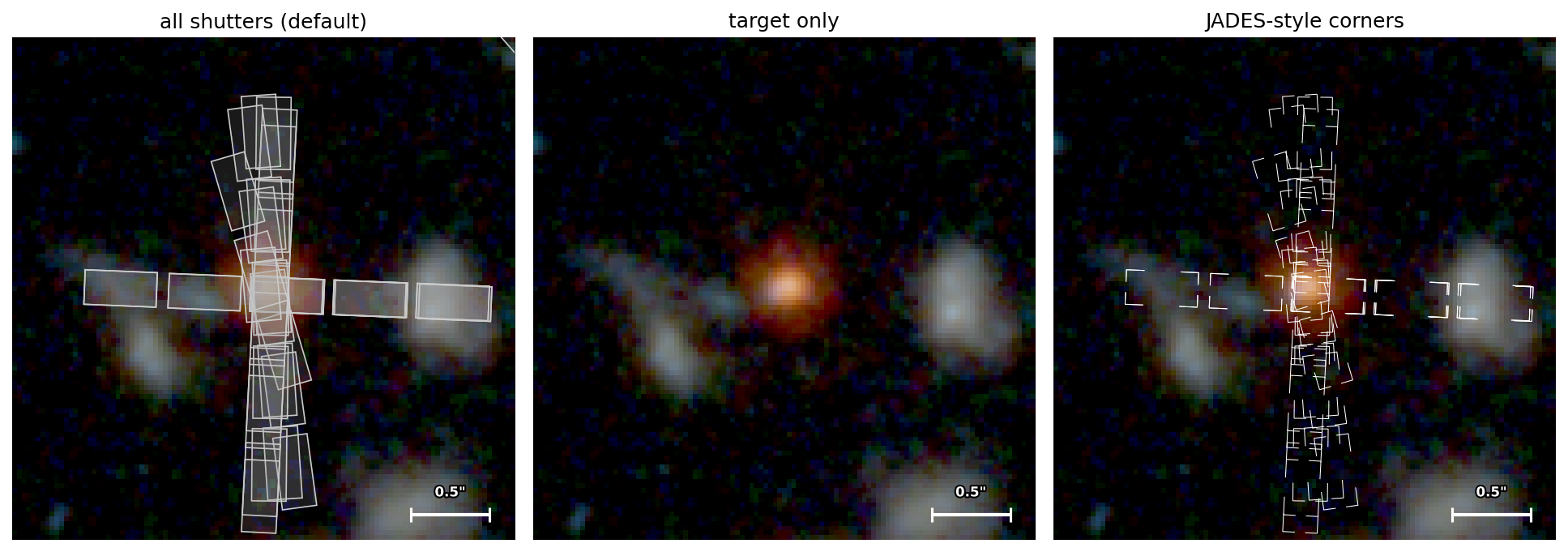
5. Publication-quality cutout#
plot_cutout() accepts a shutter_style dict to override per-category styling. Categories are 'target', 'other', and 'stuck_closed'. The marker key controls shape: 'box' (default) or 'corners' (JADES-style L-shaped marks). Partial overrides are merged with defaults.
import matplotlib.pyplot as plt
from campfire import Campfire

cf = Campfire()
fig, axes = plt.subplots(1, 3, figsize=(13, 4.5))

# 1. Default — all shutters as light boxes
cf.plot_cutout('J141934.14+525238.7', fov=3.2, ax=axes[0])

# 2. Target only
cf.plot_cutout('J141934.14+525238.7', fov=3.2, shutters='target', ax=axes[1])

# 3. JADES-style L-shaped corners with custom colors
cf.plot_cutout('J141934.14+525238.7', fov=3.2, ax=axes[2], shutter_style={
    'target': {'marker': 'corners', 'edgecolor': 'cyan', 'linewidth': 1.5},
    'other':  {'marker': 'corners', 'edgecolor': 'white', 'linewidth': 0.5},
})

fig.savefig('cutouts.pdf')   # vector shutter overlay preserved in PDF
For full control, fetch the cutout PNG and shutter JSON yourself and pass them to the underlying plotter:
from campfire.imaging import plot_cutout

path = cf.get_cutout('J141934.14+525238.7', fov=3.2)      # cached PNG path
data = cf.get_shutters('J141934.14+525238.7', fov=3.2)    # cached JSON dict
plot_cutout(path, shutters=data, object_id='J141934.14+525238.7',
            fov=3.2, ax=ax)
6. SED + spectrum overlay#
A common consistency check: overlay the broadband photometry on the spectrum. Useful for spotting calibration mismatches, slit losses, or confirming that the matched photometry catalog is the right one.
import matplotlib.pyplot as plt
import numpy as np
from campfire import Campfire

cf = Campfire()
obj = cf.get_object('J141934.14+525238.7')
spec = cf.open_spectrum('capers_egs_p3_prism_clear_11585')
phot = obj.photometry

fig, ax = plt.subplots(figsize=(10, 5))

good = np.isfinite(spec.fnu) & (spec.fnu_err > 0)
ax.step(spec.wavelength[good], spec.fnu[good], where='mid',
        lw=0.6, color='k', alpha=0.7, label='PRISM spectrum')

ax.errorbar(phot.wavelength, phot.flux, yerr=phot.flux_err,
            fmt='o', ms=8, color='C3', ecolor='C3',
            label=f'Photometry ({phot.catalog})', zorder=5)

ax.set(xlabel='Wavelength (μm)',
       ylabel=r'$f_\nu$ (μJy)',
       xscale='log',
       xlim=(0.4, 6.0),
       title=f'{obj.object_id} — z={obj.redshift:.3f}')
ax.legend()

If the photometry sits systematically above or below the spectrum, recipe 3 shows how to derive a correction curve and apply it.
See also#
- The runnable
quickstart.ipynbexecutes every recipe on this page end-to-end. - Python Client reference — every method, every parameter, organised by topic.
- CLI Reference — the
campfirecommand-line tool.